What a last two weeks it has been this semester. Hurricane Helene threatened the area during the final week of September, shifting everyone’s focus to preparation and expected impacts. The storm center passed approximately 90 miles to our west. While coastal impacts were severe, we were spared the brunt inland, even keeping electricity throughout the storm.

Followed that with a preplanned trip for AARoads to Puerto Rico. Then got started on the final module for GIS Special Topics and increased my time investment into the module leading into this past weekend as newly named tropical storm Milton formed in the Bay of Campeche. A Category 5 hurricane as of this writing, Hurricane Milton is expected to make landfall somewhere on the west coast of Florida on Wednesday or Thursday. While wind shear is eventually expected to weaken the storm, unlike Helene, Debby, Idalia and other storms, Milton is forecast to be a major wind event for inland locations. So anxiety levels are high!
 
The sixth module for GIS Special Topics investigates the effects of scale on vector spatial data and resolution on raster spatial data. The lab also covers spatial data aggregation and the concept of gerrymandering using GIS.
 
There are multiple meanings of scale to consider for Geographic Information Systems (Zanbergen, 2004).
  • as an indication of the relationship between units on a map and units in the real world. This is typically a representative fraction, which is commonly used with USGS Quads and GIS Maps in general.
  • to indicate the extent of the area of interest. Examples include spatial areas such as neighborhoods, cities, counties and regions.
  • to express the amount of detail or resolution. The resolution of a raster spatial dataset is the cell size, such as 10 meters for the Sentinel 2 blue, green and red spectral bands. This defines the scale of the data.
Scale in the Raster Data Model is straight forward represented by the resolution or cell size. A general rule is that a real world object needs to be at least as large as a cell in order to be recognizable.
 
Scale in the Vector Data Model also represents the amount of detail. While there is no single best method to express scale in vector data, a good indicator is the size of the smallest polygon or length of the shortest segment of a polyline.
 
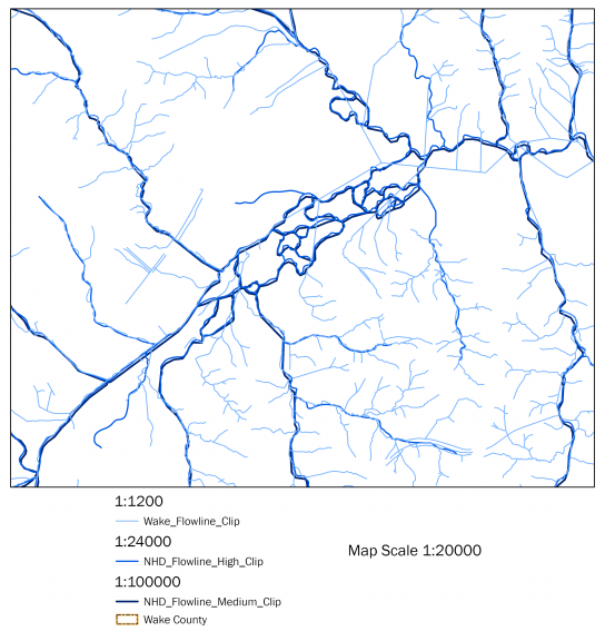
When measuring the length of a complex shape, the total length depends on the smallest unit of the measuring tool. Where the units of a measuring tool decrease, the total length of the shape increases. More nodes and connecting segments result in longer shape lengths or area perimeters. The following images illustrate the differences in scale for the Vector Data Model.
Differing scales of Wake County, NC water flowlines

Water flowline vector data for Wake County, NC in different scales

Polygon vector data for Wake County, NC waterbodies at different scales

Waterbodies vector data for Wake County, NC in different scales

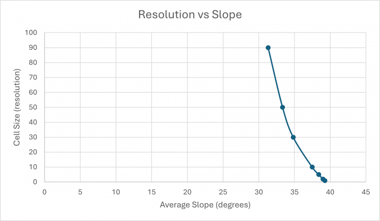
The properties of a Digital Elevation Model (DEM) depends upon what resolution is used. Higher resolution provides more detail. When measuring Slope, values decrease as the cell size increases and detail decreases. Higher detail results in steeper slopes. This effect applies to the full range of slopes regardless of steep areas of terrain (Zanbergen, 2004).

Scatterplot showing the relationship of Resolution vs. Slope in a DEM

Quantification of Resolution vs. Slope for a DEM in lab

The Modifiable Areal Unit Problem (MAUP) factors into deciding what scale to use for analysis of spatial data. MAUP is a complication with statistical analysis when quantifying aerial data. There are two facets of MAUP.
 
Scale Effect
The optimal spatial scale for analysis is generally not known, as there are multiple scales for analysis to be theoretically considered (Manley 2013). The results of data can be manipulated positively or negatively depending upon upon the size of the aggregation units used.
 
Zoning Effect
The method used to create areal units. This effect is the result of how spatial data is separated, such as the grouping of smaller areal units into less numbers of larger areal units (Dark & Bram 2007). Changing the grouping can manipulate the results of spatial analysis.
 
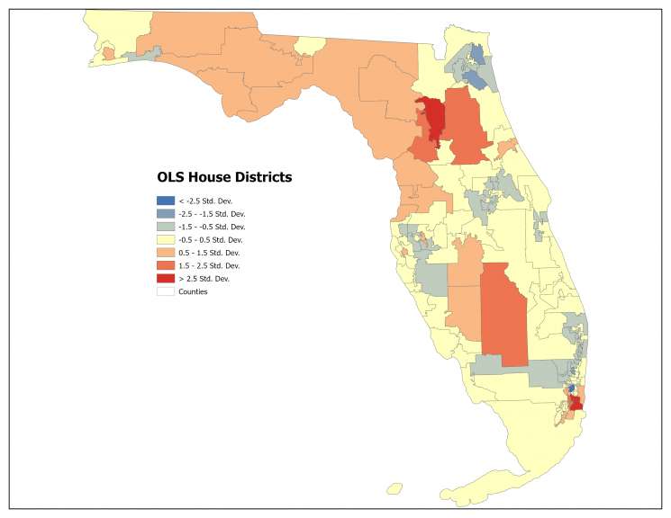
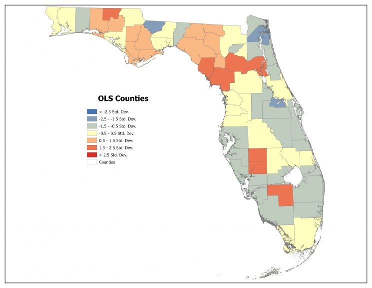
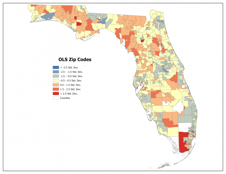
Part 2 of the lab conducting Linear Regression analysis of poverty statistics for Florida in U.S. Census data resulted in an example of MAUP. Different levels of aggregation convey different results:
Linear Regression Results based upon Congressional District

Linear Regression Results based upon Congressional District

Linear Regression Results based upon Counties

Linear Regression Results based upon Counties

Linear Regression Results based upon Zip Codes

Linear Regression Results based upon Zip Codes

Gerrymandering is the purposeful manipulation of a district shape with intentional bias (Morgan & Evans, 2018) or to affect political power (Levitt, 2010). Partisan gerrymandering takes place when the political party controlling the redistricting process draws district lines to benefit itself and restrict opportunities for opposition parties. While this maneuvering aims to increase inordinately the political power of a group (Levitt, 2010), the U.S. Supreme Court ruled that partisan-focused gerrymandering is not unconstitutional  (Morgan & Evans, 2018).
 
GIS can measure gerrymandering by the compactness in a number of ways. Compactness is the only common rule pertaining to redestricting that takes into account the geometric shape of the district. A district is considered compact if it has a regular shape where constituents generally live near each other. A circular district is very compact while a linear district is not (Levitt, 2010). 
 
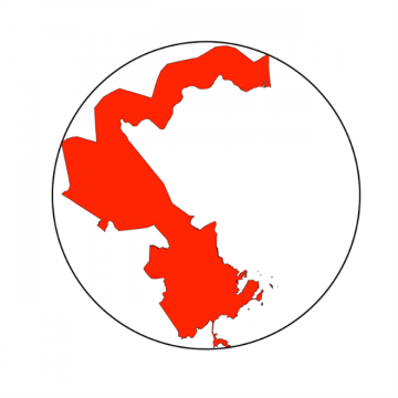
Thanks to a discussion board post from our classmate Emily Jane, a method for determining compactness that I found easy to interpret is the Reock Score. Using this method, geoprocessing determines the minimum bounding circle around each polygon of a Congressional District. That is the smallest circle that entirely encloses the district. Reock scoring uses the ratio of the district area to the minimum bounding circle with the following equation R=AD/AMBC where AD is the area of the district and AMBC is the area of the minimum bounding circle. The score ranges from 0, which is not compacted, to 1, which is optimally compact.
Example of the Minimum Bounding Circle used with the Reock Score method

An example of the Minimum Bounding Circle around a District polygon for the Reock Score method

Proceeded with the Reock Score analysis using the Minimum Bounding Geometry tool in ArcGIS Pro. This creates circular polygons for each record in the Congressional District dataset provided. With the minimum bounding circle area variable and the area value of the district, calculated the Reock score for every district. With a field added for the Reock Score, the worst “offenders” of gerrymandering based upon failing to have district ‘compactness’ from the provided dataset were determined.

Florida District 5 - 2nd worst gerrymandering 'offender'

Florida District 5 - 2nd worst gerrymandering 'offender'

North Carolina District 2 - the worst gerrymandering 'offender'

North Carolina District 2 - the worst gerrymandering 'offender'

References
 
Zanbergen (2004). DEM Resolution. Vancouver Island University, Nanaimo, BC, Canada.
 
Manley, D. J. (2013). Scale, Aggregation, and the Modifiable Areal Unit Problem. In Handbook of Regional Science. Springer Verlag.
 
Dark, S. J., & Bram, D. (2007). The modifiable areal unit problem (MAUP) in physical geography. Progress in physical geography, 31(5), 471-479.
 
Morgan, J. D., & Evans, J. (2018). Aggregation of spatial entities and legislative redistricting. The geographic information science & technology body of knowledge, 2018(Q3).
 
Levitt, J. (2010). A Citizen’s Guide to Redistricting. New York, NY: Brennan Center for Justice at New York University School of Law.