There are numerous spatial interpolation methods used to generate surfaces in GIS. This is the prediction of variables at unmeasured locations based upon sampling of similar variables at known locations or true points. Related, spatial prediction is the estimation of variables at unsampled locations based partly on other variables and a collective set of measurements. Comprised of spatially continuous data, surfaces could be topographic, a measure of air pollution, soil moisture, air temperatures and population density among others (Bolstad & Manson, 2022).
A number of factors can affect the performance of spatial interpolation methods. Some of these factors are data accuracy, temporality of the data, sampling design, sample spatial distribution, the presence of abnormal values or outliers, and the correlation of primary and secondary variables (Hu, 1995, Li & Heap, 2014).
Deciding upon the best interpolation method is not always a straight forward process. Methods often work well for a specific data set because of inherent assumptions and algorithm design for estimation. Different interpolations methods applied to the same data set may produce desired results for one study objective but not another (Hu, 1995).
Module 5 for GIS Special Topics performs interpolation analyses for Tampa Bay water quality data. Specifically four methods are used for the estimation of Biochemical Oxygen Demand (BOD) in milligrams per liter variables for Tampa Bay. A point feature class of BOD sample locations is provided and the study area is all of Tampa Bay, Old Tampa Bay and Hillsborough Bay. A statistical analysis of each is compared in an effort to determine which derived surface best describes water quality.
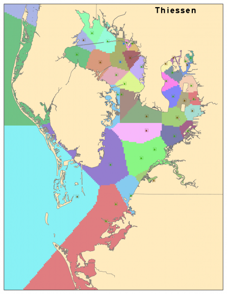
The first interpolation method implemented for the Tampa Bay water quality analysis is Thiessen Polygon. This method was the easiest to interpret. It aggregates the point dataset within the study area to polygons with one per point, which is referred to as a centroid. All estimated points within the Thiessen polygon (proximal zone) are closer in value to the associated centroid than any other centroid in the overall analysis.
The Thiessen Polygon method is optimal when there is no uniform distribution of the sample points. The method is applicable to environmental management (Wrublack et. al, 2013).
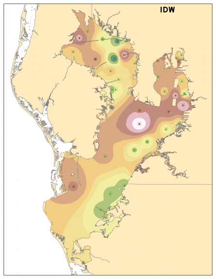
Previously discussed in the Isarithmic Mapping lab in Computer Cartography, the Inverse Distance Weighting (IDW) spatial interpolation method estimates values using the values of sample points and the distance to nearby known points (Bolstad & Manson, 2022). Values closer to a location have more weight on the predicted value than those further away. The power parameter in the mathematical equation of the method determines the weighting, which decreases as the distance increases. When the power parameter increases, a heavier weight is applied to nearby samples, which increases their influence on estimation (Ikechukwu, 2017).
The IDW method assumes that the underlying surface is smooth. It works well with regularly spaced data, but cannot account for the spatial clustering of sample points (Li & Heap, 2014).
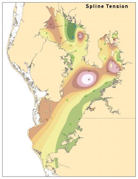
Spline interpolation uses a mathematical function to interpolate a smooth curve along a set of sample data points with minimal curvature. Polynomial functions calculate the segments between join points. These accommodate local adjustments and define the amount of smoothing. The method is named after splines, the flexible ruler cartographers used to fit smooth curves through fixed points (Ikechukwu, 2017).
The performance of Splines improves when dense, regularly-spaced data is used (Li & Heap, 2014). The method is very suitable for estimating densely sampled heights and climatic variables (Ikechukwu, 2017).
The lab uses the options of Regularized and Tension for the Spline geoprocessing tool in ArcGIS Pro. This changes the weight parameter, where higher values in Regularized splines result in smoother surfaces. A weight of zero for the Tension spline option results in a basic thin plate spline interpolation. This is also referenced as the basic minimum curvature technique.
References:
Bolstad, B., & Manson, S. (2022). GIS Fundamentals – 7th Edition. Eider Press.
Hu, J. (1995, May). Methods of generating surfaces in environmental GIS applications. In 1995 ESRI user conference proceedings.
Li, J., & Heap, A. D. (2014). Spatial interpolation methods applied in the environmental sciences: A review. Environmental Modelling & Software, 53, 173-189.
Wrublack, S. C., Mercante, E., & Vilas Boas, M. A. (2013). Water quality parameters associated with soil use and occupation features by Thiessen polygons. Journal of Food, Agriculture & Environment, 11(2), 846-853.
Ikechukwu, M. , Ebinne, E. , Idorenyin, U. and Raphael, N. (2017) Accuracy Assessment and Comparative Analysis of IDW, Spline and Kriging in Spatial Interpolation of Landform (Topography): An Experimental Study. Journal of Geographic Information System, 9, 354-371. doi: 10.4236/jgis.2017.93022.


