Continuing the focus on Spatial Data Quality in GIS Special Topics, Module 1.3 covers the Accuracy Assessment of Roads. Road networks are widely used as the basemap for many applications. This factors into expectations for positional accuracy and completeness, which this week’s lab covers.
Road networks are also used for geocoding and network routing. The usability of such is dependent upon robust attributes such as street names, address numbers, zip codes in addition to networking aspects such as turn restrictions and one-way directions. Topologically, road networks must also be robust, with exact connectivity found in reality (Zanbergen 2004).
Typically road network datasets are compiled from an array of historical sources, with digitization from aerial imagery and augmentation from GPS field data collection. One of the most comprehensive datasets in the U.S. with a long lineage is TIGER (Topologically Integrated Geographic Encoding and Referencing).
Produced by the US Census Bureau for 1:100,000 scale maps (Syoung & O’Hara, 2009), TIGER was originally compiled to be topologically correct. That is data was not focused on being as accurate as possible, but instead data stressed connections and boundaries. (Zanbergen 2004) This resulted in legacy errors, which were carried over in succeeding updates from 2000 onward.
Covered in the last week’s lab, accuracy assessment of roads utilizes methods such as “ground-truthing” using GPS or surveying equipment, comparing roads with high resolution imagery, and comparing roads to existing datasets deemed to be of higher accuracy. Positional accuracy last week looked at the comparison of points between two datasets using root-mean-square-error (RMSE) with reference or true points. Additional methods include using buffers. This is where the true line is buffered with some distance to show discrepancies. It is also used to determine where displacements between matching features fall within an expected nominal accuracy. (Syoung & O’Hara, 2009) In other words data located in areas outside a buffer (specified tolerance) are deemed to be substantial errors. Another method for positional accuracy is line displacement. This is where the displacement of various sections of a polyline are measured using Euclidean distance. Using matching algorithms, errors show the displacement of one road network from another. These displacements can be summarized (Zanbergen 2004), or be represented as a raster dataset to analyze vector geometry (Syoung & O’Hara, 2009). The lab assignment for Module 1.3 conducts accuracy assessment for completeness on two datasets of street centerlines for Jackson County, Oregon. The feature classes are TIGER road data from 2000 and a Streets_Centerlines feature class compiled by Jackson County GIS.
Completeness is one of the aspects cited by Haklay (2010) in accessing data quality. Completeness is the measure of the lack of data, i.e. how much data is expected versus how much data is present. Zanbergen (2004) references measuring the total length of a road network and comparing that to a reference scenario and secondly counting the number of missing elements as a count of features.
Both accuracy assessment scenarios for completeness overlay an arbitrary grid cell over compared datasets to determine the total length of count in a smaller unit. Then a comparison between two sets of roads based on a total length can be determined.
Haklay (2010) references completeness as asking the question of how comprehensive is the coverage of real-world objects. Generalizing this as a simple measure of completeness for our analysis, the dataset with the higher total length of polylines is assumed to be more complete.
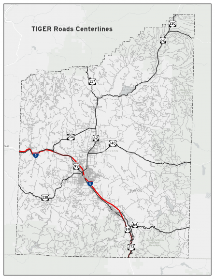
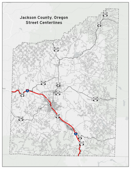
Our analysis proceeds by projecting the Tiger roads data into StatePlane coordinates to match the other provided datasets. The shape length of each polyline in kilometers is calculated from feet into a new field for each road feature class. Statistics for total length of all road segments per dataset are then summarized for the initial assessment of completeness, where the dataset with more kilometers of roads is considered more complete.
The results were 10,805.82 km of roads for the County Street Centerlines feature class and 11,382.69 km for the Tiger roads feature class. With more data, the Tiger roads data is considered more complete.
Further accuracy assessment for completeness continues with a feature class of grid polygons to be used as the smaller units for comparison. Both feature classes were clipped so that all roads outside of the 297 grid cells were dropped. Geoprocessing using the Pairwise Intersect tool separates each road centerline dataset by grid. This provides a numerical summary indicating a simple factor of completeness on a smaller scale.
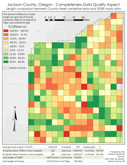
The collective length of Tiger road segments exceeds the County street centerline segment length in 162 of the 297 grid cells.
The collective length of County street centerline segments exceeds the Tiger road segment length in 134 of the 297 grid cells
Additionally one grid cell contained zero polylines for either centerline dataset.
Visualization of these results shows the percent difference for the length of Tiger roads centerline data as compared to the County roads centerline data. Statistics were calculated using a mathematical formula:
% = ( ℎ − ℎ )/( ℎ ) ×100%
Completeness is aggregated where cells with more kilometers of Tiger roads than County roads appear in reds and oranges and shades of green where the collective length of County roads polylines exceeds the length of the Tiger roads data.

Map showing the geographic distribution in the differences of completeness for the two road datasets
References:
Zanbergen (2004, May). Spatial Data Management: Quality and Control. Quality of Road Networks. Vancouver Island University, Nanaimo, BC, Canada.
Suyoung & O’Hara (2009, December). International Journal of Geographical Information Science 23, 1503-1525.
Haklay (2010, August 1). Environment and Planning B: Planning and Design, 37, 682-703.


