
The sixth lab for Intro to GIS introduces Georeferencing, which transforms raster data such as an aerial photo or a scan of a subdivision plat, to closely match vector data within GIS. I am familiar with Georeferencing from my cartography jobs, where we often acquired subdivision and other development plats and digitized them for updating map products.
Georeferencing utilizes control points, which match features on the raster image without any location data (coordinate system, latitude/longitude), to an existing vector data set in GIS. There are multiple methods of transformation with Georeferencing. The type of transformation used determines the correct map coordinate location for each cell within the raster data.
A lower order transformation, such as Zero Order Polynomial is used to simply shift data to better line a raster image with vector data. This is often the case if the spatial accuracy of the raster is similar to the vector data, or if the raster image was previously georeferenced and needs slight tweaking of its location to better match vectors. Correcting more complex distortion, higher order transformations allow raster data to bend and warp more.
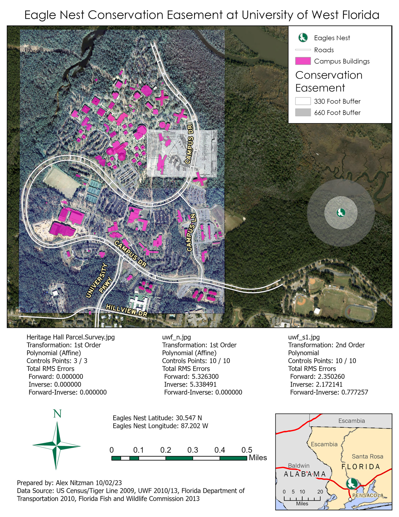
This week’s lab georeferences two aerial photographs of the University of West Florida (UWF) campus to feature layers for campus roads and buildings. I utilized a First-Order Polynomial transformation on the north aerial of the campus. First-Order is used to affine transformation to shift, scale or rotate raster data. Affine is defined in mathematics as “allowing for or preserving parallel relationships”, so it more or less in this case scaled the raster image down to match the vector data without much in the way of distortion.
The south aerial of the UWF campus utilized a Second-Order Polynomial transformation. This was due to the aerial being intentionally distorted. Needing at least six control points, second order transformation is used where a raster dataset must be bent or curved to line up with vector data. We used ten control points.
Root Mean Square (RMS) Error was also introduced in this week’s lab. RMS calculates the difference between where the from point was ultimately located opposed to the actual location specified. The value describes how consistent transformation is between the different control points. We were looking for RMS values of less than 15, any points exceeding that were beyond the accuracy tolerance.
With georeferencing completed, I added a line feature for Campus Lane, a new road constructed since the original data was processed in 2010. I also digitized the new UWF gym, Building 72. With these features added, our next step was to introduce a multi-ring buffer around a nearby Eagles nest, a protected species. Located in an undeveloped area within UWF land to the east, our analysis added 330 foot and 660 foot buffers around the nest location representing two levels of conservation easement. These easements could affect construction of new buildings as part of planned expansion of the UWF campus.
The finished aerial map juxtaposes the existing UWF campus building structures with the conservation easement around the known Eagles nest location.

Leave A Comment